Posts: 236
Threads: 26
Joined: Mar 2020
Reputation:
29
Operating system(s):
- Windows (Vista and later)
Gimp version: Don't know yet
I return to my old love: parametric curves. You may remember that I wrote a plugin to draw parametric curves as Gimp's paths approximately. Now the plugin has a new version. It is so big overhaul that I prefer to start a new thread. I wish everybody would just forget the old one.
The new version 2.1 has a new approximation algorithm. Meanwhile I have learned something about plugin writing, and I also had my eye on how the extension Parametric Curves is done in Inkscape, and I hope that I now managed to make my plugin a little more user-friendly. Anyway, it is no longer so loaded with options nobody wants.
If you have in your plugins folder files 'parametric_curves.py' and 'simple_parametric_curve.py', please delete those. To get the new version (2.1), click the link
http://kmarkku.arkku.net/Parametric_curv...aster.html
scroll down and download the file for Parametric curves; this gives you the .zip file parametric_curves_2_1.zip. (There is another download button for Special curves, an update of an old version, but I talk now only about the Parametric curves.)
The .zip file parametric_curves_2_1.zip contains one file parametric_curve.py and a small file doc.pdf. When you unzip the .zip file and move the .py file to your user's plug-ins folder, and restart Gimp, you find in the menu at
Filters > Render > Parametric curves
three plugins:
- Parametric curve (cartesian)
- Parametric curve (polar)
- Parametric curve (read function from file)
The documentation file doc.pdf contains explanations and instructions. They are probably useful only if you try the third plugin. Otherwise you don't lose much if you skip the documentation and just go experimenting.
The first plugin is the basic form, and I talk only about that in this post. The other two I shall explain later.
Open the first plugin Parametric curve (cartesian). If you let the default values in the GUI be as they are and just press OK, you get a half circle, as large as can be fitted on the screen. I don't show it here: you know what a half circle is.
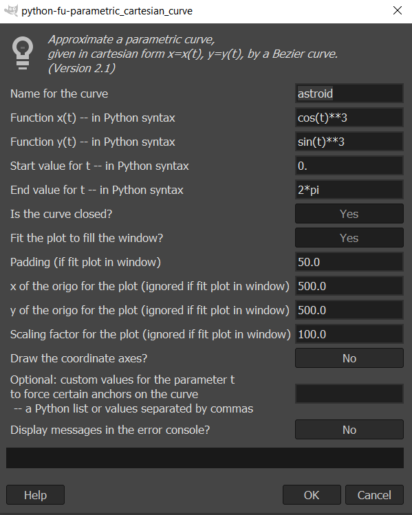
To get a better example, put in the GUI the following:

Changes from the defaults are:
name = astroid
x(t) = cos(t)**3
y(t) = sin(t)**3
start value for t = 0 (this is the same as default)
end value for t = 2*pi
the curve is closed
padding = 50
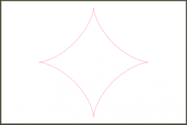
Then on the screen you get an astroid, fitted to fill the screen with a little padding. And it is a path, so all stroking is left to the user.

That is the idea. If you keep 'fit to window' as Yes, you get as large a curve as fits on the screen and the next field enables you to put some padding. But clicking 'fit to window' to No, you can control the size and placement with the three inputs 'x of the origo', 'y of the origo' and 'scale'.
<...skip on first reading...>
There is one input which you can usually safely just ignore: custom parameter values. But I explain the idea for once: Consider the astroid example. There are four cusps. The plugin puts one anchor at each cusp. Those anchors should be set rather precisely to obtain a faithful rendering of the astroid. But how does the plugin find the cusps? It cannot compute derivatives (which would bring the problem down to solving equations). No, the only thing it can do is to run along the curve and examine it at very many close points. That is what it does and that is how it finds cusps (or inflection points or whatever). You understand that that is necessarily inaccurate. So, the idea in those custom points is that the user can help the plugin in its work. The user can list the parameter values (pi/2, pi, 3*pi/2) which give three of the cusps (the fourth is the starting or ending value of t, so the plugin knows it anyway). When the plugin is given those exact parameter values it places anchors at those exact spots and the result will be more accurate.
But in its current form the plugin is so good in finding cusps on its own (or inflection points or whatever) that you can usually ignore this difficulty. But it is good to know just in case: with custom points you can force the plugin to place anchors at some particular points. Then those points will be exactly on the right curve. Between the anchors the curve will only approximate the true curve.
</...skip on first reading...>
You may recall that the goal of this plugin is: Given a parametric curve,
1. approximate it with a path (a composite Bezier curve);
2. try to do this very accurately; and
3. do this with only a small number of control points.
Requirements 2 and 3 are contradictory, but at the moment I am rather pleased with how the plugin works.
If you try the plugin with complicated curves you are likely to find trouble cases where something goes wrong. I shall be grateful if you report those: the functions, the interval, custom points (if any), and any error messages.
Posts: 236
Threads: 26
Joined: Mar 2020
Reputation:
29
Operating system(s):
- Windows (Vista and later)
Gimp version: Don't know yet
I say now something about the second plugin Parametric curve (polar). It draws curves given in polar form r=f(t) where t is the argument angle (the angle from the positive x axis).
The default values draw a piece of the logarithmic spiral r=exp(t/10). The default start and end values of t are 0 and 4*pi and with those you get 2 rounds of the spiral.
By changing the inputs you can get shorter or longer parts of the spiral. Inputs r(t)=exp(t/20) and start t = -10*pi and end t = 10*pi give a tighter and longer logarithmic spiral:

I used here the default value "fit in the window" = Yes with a little padding, to get the curve fit nicely on the screen.
As another example, the blue curve on the left below is the cardioid. It was drawn with r(t)=1-cos(t), and the start and end value of t are 0 and 2*pi. Also, the curve is closed, so in the GUI it is good to set "closed" to Yes.

Just to try something else I changed r(t) to (1-cos(t))*sin(t). The result is on the right. I don't know if the curve has any name.
These plugins are now so good and easy that you can go experimenting. It is fun. And even better is the third plugin where the function (and perhaps some other data) is read from a file. I shall explain that in the next post. Tomorrow. But best it is explained in doc.pdf, and there are two examples, so you can already try it yourselves.
Posts: 236
Threads: 26
Joined: Mar 2020
Reputation:
29
Operating system(s):
- Windows (Vista and later)
Gimp version: Don't know yet
Now I show how to use the third plugin Parametric curve (read function from file). The details are explained in doc.pdf, so if you are interested, please read it. I show here two examples. The file doc.py contains two other examples.
I don't do much explanations here. For more details and better explanations, please look at doc.pfd.
The GUI is almost the same as for the other two plugins, but instead of functions x(t), y(t), or r(t), it asks for a file.
Example 1: The cochleoid
To follow this example, make a file with the following contents. Note that it must be valid Python code, so care must be taken of indentations for example.
Code:
def function(t):                   # cochleoid

    from cmath import exp as cexp

    try:

        r = sin(t)/t

    except ZeroDivisionError:

        r = 1

    return r*cexp(1j*t)


curve_name = 'cochleoid'

interval = [-10*pi, 10*pi]

closed = False
Save the file as somefile.py to somewhere where it is easily found (desktop perhaps). Open the GUI of the plugin, and there choose the file somefile.py. Press OK. If everything is ok you get the following curve, called the cochleoid:
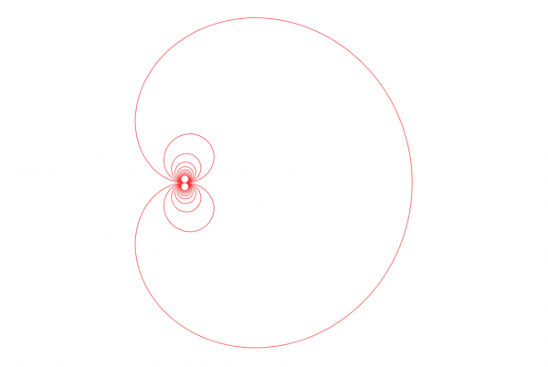
Explanation: The file is valid Python code. There "def function(t):..." implements the function for the cochleoid curve. The "interval = ..." defines which part of the curve will be drawn.
In the definition of the function, I mention a couple of points for those interested: The function must return a complex number (the plane is viewed as the complex number plane). The defining equation for the cochleoid in polar form is r=sin(t)/t. In the code the factor "*cexp(1j*t)" converts it to proper complex-valued function. The exception ZeroDivisionError occurs when t=0, and there the limit value sin(t)/t -> 1 is used.
Example 2: Experimenting
The formula for the cochleoid in polar form is r = sin(t)/t where t is the argument angle (or polar angle = angle from the positive x axis).
Quite by chance I happened to see yesterday a similar formula r = sin(n*t)/sin(t) while surfing in search of something else. Since I now have this system which makes it easy to experiment with such formulas, I had to try this one. I wrote the following piece of code in a file:
Code:
n = 7 # integer > 0


def function(t):

    from cmath import exp as cexp

    try:

        r = sin(n*t)/sin(t)

    except ZeroDivisionError:

        r = n*cos(n*t)/cos(t) # limit by l'Hospital

    return r*cexp(1j*t)


curve_name = 'experiment n='+str(n)


if n%2 == 0:

    interval = [0,pi]

else:

    interval = [0,2*pi]


closed = True
Here n is a parameter, a positive integer. To change it I have to edit it in the file. When we vary n, the curves follow two patterns. With odd n the curve is symmetric both in x and y directions, but with even n the symmetry in x direction is lost. A typical odd case is given by n=7:

The larger n, the larger the number of petals. This looks nice, don't you think? I can imagine that from these one could build a pretty ornament. And it is a path, so the user is free to choose any stroking.
If you have any questions, just ask. Notice that this plugin enables you to write complicated functions since you have free hands to do any Python coding. But it may happen that the plugin cannot handle all inputs. It is written by me, after all, and I am not much of a coder, and since I know the inner structures of the plugin with all those ad hoc solutions and fine-tunings, I know that much can fail. If you run into troubles with the plugin, I would be interested to hear about it.
Posts: 236
Threads: 26
Joined: Mar 2020
Reputation:
29
Operating system(s):
- Windows (Vista and later)
Gimp version: Don't know yet
That will suffíce about the general-purpose plugins for now. I talk now about the plugins which draw some special curve.
I updated the plugin file special_curves.py. It is now version 1.7. To get it, go to
http://kmarkku.arkku.net/Parametric_curv...aster.html
scroll to the bottom and download. That gives you a .zip file. Unzip it and put the file special_curves.py in you Gimp's user's plug-ins folder and restart Gimp. You will find at
Filters > Render > Parametric curves > Special curves > ...
five plugins:
Fourier3 with control of symmetry
Fourier3
Lissajous
Rhodonea
Spiropath
The two Fourier plugins are new; of them I shall talk later. In this post I talk about the old three. And I am not doing any talking. I just show pictures to remind what the they can do. (And these are just some random examples that I happened to make.) To get a particular curve, I have no advice about how to find proper inputs. One just has to experiment.
Lissajous
The input parameters I used are shown in the picture.
 Rhodonea (the rose curve)
 Spiropath

These were made with the following inputs:
1: 30, 11, 0.9
2: 30, 11, 0.5
3: 30, 26, 1 fixed circle not drawn
4: 11, 2, 0.5 epitrochoid
5: 11, 5, 0.7 epitrochoid
6: 30, 26, 1 hypotrochoid
7: 3, 1, 0.9
8: 6, 11, 1 hypotrochoid
9: 11, 5, 1 fixed circle not drawn
10: 6, 5, 0.5
Posts: 236
Threads: 26
Joined: Mar 2020
Reputation:
29
Operating system(s):
- Windows (Vista and later)
Gimp version: Don't know yet
I explain now the plugin Fourier3. (The other one, "Fourier3 with control of symmetry" will be in turn later.)
If you run the plugin Fourier3 with the default values you get the figure on the left:

That curve was not my invention. I took it from a writing by Frank A. Farris:
https://scholarcommons.scu.edu/cgi/viewc...th_compsci
which you may wish to glance at (it is mathematics but there are some pretty pictures). The idea in the plugin is pure mathematics but when you try to get some understanding of what the plugin does it is better to think as follows:
Look at the drawing on the right above. Or look at Figure 1 in Farris's paper; it is clearer. Now imagine the following: We have three wheels. The largest has its center fixed and it revolves around the center with some constant rate. The second wheel has its center attached to some point on the perimeter of the first wheel, so it follows along when the first wheel revolves. At the same time the second wheel revolves at some constant rate around its own center. And the third wheel is attached to some point on the second wheel's perimeter, and it too revolves at some constant rate. And then there is a pen attached to the third wheel's perimeter. That pen draws some curve (the dashed curve above) when the wheels revolve.
Can you imagine that? Can you see the wheels going round and the curve to be drawn? It is difficult, and I wish I could make an animation of it. But you can look at the first half minute of the video
https://www.youtube.com/watch?v=r6sGWTCMz2k
There there are many more wheels than 3, but it gives the idea.
So that is the best way to think about it, but if you know some mathematics you can think of it as the first 3 terms of a complex Fourier series. That explains the name "Fourier3" of the plugin.
You may remember that the spirograph has two wheels going round. Here we have three. Indeed, what the spirograph draws can be drawn with this Fourier3 plugin too, though the connection is not obvious or easy. And even the rhodoneas (rose curves) can be drawn with Fourier3. In this sense, Fourier3 generalizes both of my Spiropath and Rhodonea plugins. But those two may be easier to use.
The main inputs to Fourier3 are:
- three "frequencies"
- three "coefficients".
Those words refer to the Fourier series, but when we think of the wheels, the "frequencies" are the revolving rates of the wheels, and the "coefficients" are the radii of the wheels. With that info you may try to understand how the plugin works.
(Just for completeness sake: The coefficients are usually floats, but you may also input complex numbers. The complex parts cause phase shifts to the wheels. Never mind about that now. You can just use floats; then all resulting curves will have vertical reflection symmetry.)
When one starts to use Fourier3, the main impression is that it is rather frustrating. It can draw pretty curves, certainly. But the inputs are complicated (3 integers and 3 floats or complex numbers). And if you have in your mind some particular kind of a curve, in practice there is no way to know from beforehand what would be good inputs. The only way to use the plugin is to keep trying with different inputs, and if you happen to get some pleasing picture, grab it and save the inputs for later use. This is something I cannot help. I have no more insight to this problem.
To save the inputs you need not write them down: If you run the plugin with the last input "Display messages" set to "Yes", there will be messages in the error console, including suitable inputs to make that curve (possibly a little different from what you used). You can copy those to a file.
Varying coefficients
In these three figures I used the same frequencies (2,-3,-18) but I made little changes in the coefficients:

The path on the left I got with with the default coefficients (1, 0.5, 0.25). The second figure was made with otherwise the same inputs except that I changed the third coefficient from 0.25 to 0.125. That little change made the curve rather different. But that I couldn't guess from beforehand! There is no way but to try different inputs and to see what comes. The third figure was made by the same frequencies but with coefficients (1, 0.25, 0.125), a little change in the second coefficient.
About rotation symmetry
Why the default figure (first picture) has 7-fold rotation symmetry and the other three (second picture) have 5-fold symmetry? It can be explained. It is solved in the nice theorem by Farris (in the site mentioned above); look there if you want to see the rule precisely. For anybody curios, I say now just this: In these examples, in the first picture the frequencies (2,-5,-19) are all of the form 7q+2 for some integer q. In the second picture the frequencies (2,-3,-18) are all of the form 5q+2. Note the 7 and the 5.
So, it is the frequencies that dictate the rotation symmetry.
Varying frequencies
Three examples with the default coefficients (1, 0.5, 0.25) but with different frequencies:

The frequences are, respectively, (1, -8, -35), (1, -10, -32), and (1, 4, -11), hence the symmetries are 9-fold, 11-fold, and 3-fold (Farris!).
The next plugin "Fourier3 with control of symmetry" makes it easier to obtain some desired symmetry. That also makes experimenting a little more efficient. I explain that in my next post.
Posts: 236
Threads: 26
Joined: Mar 2020
Reputation:
29
Operating system(s):
- Windows (Vista and later)
Gimp version: Don't know yet
I explain now the plugin "Fourier3 with control of symmetry". In it I implemented Farris's theorem (see the previous post) to give the user easy control of the rotation symmetry. You can make a curve with m-fold symmetry by inputting m in the plugin.
(And it would be very nice if other features than rotation symmetry could be controlled so easily. Alas, I don't know any counterparts to Farris's theorem concerning other features. And that theorem I happened to find quite by accident when I was looking for something else.)
The GUI is similar to Fourier3 but there are three more inputs: m, k, and a boolean input.
If you put, say, m=5, the plugin takes your inputs for frequencies and coefficients, and modifies the frequencies so that the curve will have 5-fold rotation symmetry.
That input k can be used to get some variation: different values may give even drastically different shapes (though sometimes changing k will change nothing). But the real variation comes from your input frequencies and coefficients. (The reason for such k is that it appears in Farris's theorem, and I didn't find any better way to get a value for it but to let the user to input it. You can just let it be k=1 if you like.)
The boolean input asks if you want to retain any symmetry that may be inherent in your input frequencies. Example: Suppose that you write in the GUI the frequencies (2,-5,-19). Those would give rise to 7-fold symmetry in Fourier3 (Farris's theorem!). Suppose that you now input m=5. If the boolean input is "No", the plugin demolishes that 7-fold symmetry and you are given a curve with 5-fold symmetry. But if the boolean input is "Yes", the 7-fold symmetry is preserved and you get 35-fold symmetry. Naturally, that is what you get when you have both 7-fold and 5-fold symmetries in the same figure.
(More precisely, the rule goes like this: Let M be the symmetry contained in your frequencies (above M=7). If the boolean input is "Yes", the plugin gives Mm/gcd(M,m)-fold symmetry (where gcd means the greatest common divisor). Namely, Mm/gcd(M,m) is the smallest positive integer divisible by both M and m.)
I think that this plugin is better for experimentation than Fourier3 since you can determine the rotation symmetry. On the other hand, if you for some strange reason have some 3 frequencies and you want to see what kind of curves you get with them, then use Fourier3; that plugin keeps faithfully your frequencies.
When you find inputs that make a nice curve and you want to be able to re-create the curve at some later time, do the following: Re-run the plugin with "Display messages" set to "Yes". Then in the error console you find (among other things) values for Frequencies and Coefficients which, when inserted in Fourier3, produce that curve. You can copy those values to some file and save.
As an example on varying k, below are the curves I got with default frequencies and coefficients but setting m=5 and the boolean input to "No", and tried different values for k. Here are those that pleased the eye: k=1,2,3,4 and k=-1,-2,-3,-4. Note the 5-fold symmetry everywhere.

(And please do not ask how m and k work precisely. The rules I coded into the plugin are ad hoc, to say the least. They may change if ever get some better ideas.)
The same exercise with frequencies (1,4,7), m=5, and k=1,2,3,4:

Posts: 1,165
Threads: 179
Joined: Sep 2018
Reputation:
115
Operating system(s):
- Windows (Vista and later)
Gimp version: 2.10
Nice done, a little flower grown from this plugin :

Posts: 236
Threads: 26
Joined: Mar 2020
Reputation:
29
Operating system(s):
- Windows (Vista and later)
Gimp version: Don't know yet
Nice, though a little small. Here is another. This is based on a path which can be made in Fourier3 with Frequencies=(1, 13, 25) and Coefficients=(1, 1.2, 1). (I don't remember which of the two Fourier plugins I used originally.) Then it was just applying path to selection and playing with a gradient and curves. And bucket fill and making the background.

Posts: 1,538
Threads: 71
Joined: May 2021
Reputation:
167
Operating system(s):
Gimp version: 2.10
A quicky made with "Fourrier3 with control of symmetry" default values (I'm gonna love those parametric paths)

Posts: 1,165
Threads: 179
Joined: Sep 2018
Reputation:
115
Operating system(s):
- Windows (Vista and later)
Gimp version: 2.10
Ottia Tuota and PixLab, nice to see your artistic skills. As PixLab mentioned, parametric paths by Ottia Tuota, a new challenge to work with. Here some simplistic art Piet Mondriaan style.

|
